

This Cleaning Memo is a continuation of the discussion in the July 2022 Cleaning Memo. Please review that before you continue with this Month’s Cleaning Memo. In this continuation we will cover the issue of histograms to provide a one-time picture of the health of cleaning validation data. It is assumed that the data generated is for cleaning of a specified product on either a single equipment item or on an equipment train. Combining data from different equipment or from different cleaned products may be an interesting exercise for other reasons, but it is not appropriate for the focus here. Combining data from different cleaned product would be like combining data from different manufactured products for process validation; it is just not assessing data that represents the same population.
So, in this Cleaning Memo we will discuss the use of histograms to give use a snapshot of our cleaning validation data and therefore of our cleaning validation program. A histogram is a bar chart with data, such as measured residue data (M4, as given in the June 2022 Cleaning Memo), with taller bars based on greater frequency. They are sometimes called “bar charts”. What will be done is to take the data from the five examples used last month, present the data as histograms, and then discuss the implications.
Example #1:
In this example, I have fifty swab results. Of those, twenty are 1.0 mcg/swab, ten are 2.0 mcg/swab, and twenty are 3.0 mcg/swab. My cleaning validation limit (calculated from a carryover equation) is 10 mcg/swab (this is the USL). The calculated mean is 2.0 mcg/swab, and the calculated SD is 0.90 mcg/swab. Using the equation given last month, the Cpu is 3.0. Here is that data presented in a simple histogram, with the limit of “10” marked with a dashed line:

In this situation, the data are all “well below” my acceptance limit, and while not a normal distribution, I should not expect a normal distribution because the locations selected are generally worst-case locations, not statistically based locations. I am happy.
Example #2:
In this example, I also have fifty swab results. Of those, forty seven are 1.0 mcg/swab and three are 5.0 mcg/swab My cleaning validation limit (from a carryover equation) is 10 mcg/swab. The calculated mean is 1.2 mcg/swab, the calculated SD is 0.90 mcg/swab, and the Cpu is 3.0. Here is that data presented in a simple histogram, again with the limit of “10” marked with a dashed line:
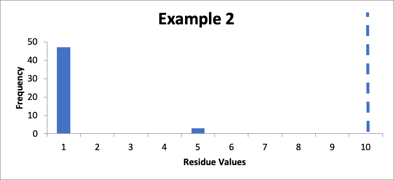
As discussed last month, compared to Example #1 the lower mean and the same Cpu in Example #2 do necessarily mean I should be happy with these results. While it does mean I meet my acceptance criterion, the three higher data values should be of some concern. I should consider evaluating the sampling locations of those three higher results to see if there is anything about any of those locations that suggests a need to improve my cleaning process. For example, if all three higher results are from the same sampled location (perhaps on cleaning of three different drug product batches), then corrective or preventive action might be taken (either to lower the measured values for those locations or to prevent those measured values from going much higher). While the Cpu value is interesting, it gives me a less useful picture of what is going on.
Example #3:
In this example, I also have fifty swab results. Of those, forty nine are 1.0 mcg/swab and one is 8.0 mcg/swab My cleaning validation limit (from a carryover equation) is 10 mcg/swab. The calculated mean is 1.1 mcg/swab, the calculated SD is 1.0 mcg/swab, and the Cpu is 3.0. Here is that data presented in a simple histogram, again with the limit of “10” marked with a dashed line:
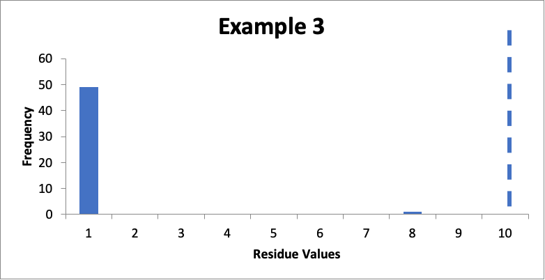
Compared to Example #2, the lower mean and the same Cpu mean does not mean I should be happy with these results. While it does mean I meet my acceptance criterion, that one higher data value of 8.0 mcg/swab should raise significant concerns. I should probably pay more attention to that one sampling location (for example, if this is data from multiple batches, what were the results for that sampling location for other batches). Collecting more data on additional batches may help alleviate concerns if subsequent data is all closer to 1.0 mcg/swab, or that additional data may point to a significant issue with that specific sampling location. This would be another case where a Cpu is interesting, but is probably not as critical or useful for establishing the “health” of the data.
Example #4:
In this example, I have fifty swab results. Of those, ten are 1.0 mcg/swab, ten are 2.0 mcg/swab, ten are 3.0 mcg/swab, ten are 4.0 mcg/swab, and ten are 5.0 mcg/swab. The cleaning validation limit (from a carryover equation) is 10 mcg/swab. The mean is 3.0 mcg/swab, the calculated SD is 1.4 mcg/swab, and the Cpu is 1.6. Here is that data presented in a simple histogram, again with the limit of “10” marked with a dashed line:
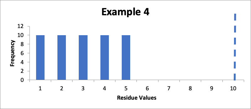
While this Cpu is much lower than in the other examples, it is still what is generally considered a “good” Cpu value. However, despite that Cpu value I would probably want to improve my cleaning, not because of any concern with the statistical consistency of the process, but rather because of a concern about the robustness of the cleaning process. Other things being equal, I generally teach that the goal in the design of a cleaning process should be to have measured values that are in the range of 20% (or below) of the calculated limits, thus clearly demonstrating the robustness of the cleaning process.
Example #5:
In this final example, I also have fifty swab results. Of those, four are 7.0 mcg/swab, forty two are 8.0 mcg/swab, and four are 9.0 mcg/swab. The cleaning validation limit (from a carryover equation) is 10 mcg/swab. The mean is 8.0 mcg/swab, the SD is 0.4 mcg/swab, and the Cpu is 1.6. Here is that data presented in a simple histogram, again with the limit of “10” marked with a dashed line:
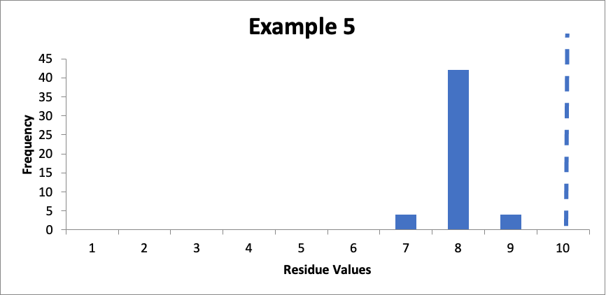
The Cpu in this case is the same (1.6) as for Example 4. However, it should be clear that the data in Example #4 is much preferable, which suggests that Cpu alone is not the best indicator of the “health” of a cleaning validation program. This Cpu is still what is generally considered a “good” Cpu value. However, despite that Cpu value I would probably want to improve my cleaning, not because of any concern with the consistency of the process, but rather because of a concern about the robustness of the cleaning process.
In these histograms I have provided, the data is always a full integer, which in most cases does not reflect actual situations. While it certainly possible to use specific reported data as the intervals (such as 1.1, 1.2, 1.3, 1.4, and so on), another option is to create “bands” for the histogram intervals. For example, any samples with values between “not-detected” up to <1.5 mcg/swab are banded together as “1 mcg/swab”, those from 1.5 mcg/swab up to <2.5 mcg/swab are banded together as “2 mcg/swab”, and so on. How the bands are selected requires judgment on the part of the scientists involved so that useful insight can be obtained.
My belief is that the evaluation of such data from different sampling locations using histograms to provide a snapshot (a one-time picture) in combination with trending of data (to be covered next month) is a better assessment method to determine the overall “health” of cleaning validation data (at least as compared to just the use of Cpu calculations). Realize also that there may be other assessments (such as deviation management, change control, and training) that should be considered to evaluate the overall health of your cleaning validation program.
As mentioned last month, I should also repeat that I am not a statistician.
Copyright © 2022 by Cleaning Validation Technologies